A geochemist studies the distribution of the 100-odd elements that form the primary building blocks of the known universe, especially those occuring in the rocks and minerals of the earth's lithosphere, hydrosphere, biosphere and atmosphere. Where possible study is also made of the composition of moons, meteorites, other planets and suns. He also strives to form theory to logically explain the element distribution found. Every one of our 92 + approx. elements plays some vital role in the technological age, and where no element has exactly the properties required of a material, marvels can be wrought by the formation of alloys and new molecules. Our list of construction materials is thus almost limitless and needs to be. Every single thing we eat, wear, live in, travel in and drink coke out of was primarily derived from the ground beneath our feet. It does occur to some of us, that geochemistry is THE primary science.

The Objectives of GEOKEM

With the amount of data being produced in the fields of Petrology and Geochemistry, we find that any statement or summary made more than two years ago is already greatly in need of revision. Nor can students being expected to read and remember the thousands of papers and publications produced annually. Approximately 4000 scientific papers likely to have some relevence to geochemistry were published in the last 12 months. The compilation of abstracts for the 2005 Fall AGU meeting included about 10,000 abstracts, mainly poster sessions. There has been no summary of the composition of the Hawaiian Islands written in the last 30 years, and no overview of the Oceanic crust, which constitutes 60% of the Earth's surface has ever been written. Even "Geokem" has far less on Oceanic sediments that we would like though we can clain a fairly complete coverage of Oceanic basalts. Due to the well known phenomena of mental inertia, outdated theory which has become fashionable or politically correct often cannot be questioned twenty years or more after it has become plain that it is not adequate so progress in knowledge is much slower than it should be.

GEOKEM aims at keeping at hand and referable to within seconds, a brief description of the composition of all volcanic and igneous centres world-wide (and some associated sediments) for which there is reasonable data, together with a regional variation diagram as well as a multi-element fingerprint, REE, metals, the alkaline earth trace elements (Zr, Nb, Sr, Rb, Y, Ba) and other relevant diagrams for single centres. Short descriptions together with fractionation diagrams, comparisons between the different types of basalt known as ORB (Oceanic Ridge Basalt), NMORB, EMORB, OIB, IAB, CAB, (see Glossary for terminology) and other fundamental magma types, graphic comparisons between centres of similar and dissimilar type, and the primary basaltic parental magma trends and fractionation trends etc are all shown. It is continuously updated as new data comes to hand. There are still omissions, diagrams not yet done etc due to lack of finance and that ever scarce commodity, time. All data used has been identified by an abbreviated reference, necessarily so, as it must fit in the width of a computer plot. If any data used is missing a reference somewhere in the general text, we welcome communications pointing this out. Completed references to all published data are also to be found in the main databases PETDB and GEOROC and sometimes we show copies of these.
We show about 1200 diagrams and more than 240 illustrating pix but these are very hard to come by for places we have not visited personally.

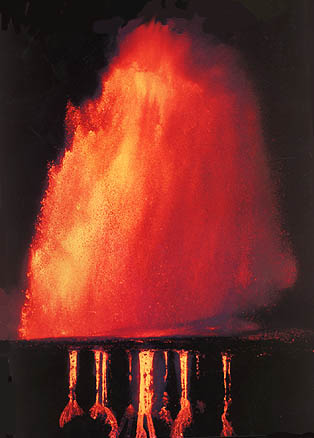
In addition surveys are given of the more important elements, their fractionation paths, their distributions in major rock types, where the greatest abundance's are likely to be found, and their ratios to related or similar elements and their current industrial consumption levels and cost. However, it is unlikely this will ever be completed for all 100 elements, however desirable this may be, for sheer pressure of time and due to the fact that some are present only in ppb (parts per billion) levels so that analysis is very difficult and data scarce. Most of the published Sr87/86, Nd143/144 and Pb 204-206-207 and 208 isotopic data are also shown.

Most of the data used can now be found in the two new databases PETDB (sea-floor basalts); GEOROC (continental and oceanic island rocks, and the still incomplete NAVDAT which covers continental volcanic rocks of Canada, Western USA and Mexico, unconnected with recent subducting continental margins. Thanks are also extended to those research workers who have over many years, forwarded both pre-publication and copies of published data. We welcome reprints of such data or .pdf files when available in order to update references.

Bearing in mind the many graduate students who may undertake a research project in this field without having been fortunate enough to have seen a recent volcano, or an eruption, we have tried to illustrate the centres described. Few could deny that the illustration of the semi- submerged Deception Island by Dr John Smellie of BAS, or the remarkable view of the explosive 1994 eruption of Mt Ruapehu, NZ, by an unknown photographer, lend an interest that would otherwise be quite lacking. Pix of similar standards are always more than welcome but the extreme reluctance of institutions, Volcano Observatories etc to let others see pix and illustations they may have is one of the biggest handicaps we face, so our illustrations are seldom to the standard we would like.
In places attention is drawn to the conspicuous lack of recent data for some well known and critical centres and volcanic islands, among which could be numbered Gough and Tristan da Cunha. For these, the most potassic basaltic centres known, in spite of the excellent pioneering work on Anton le Roex and Tony Erlank, we have little in the way of REE or other data for elements such as Tl, Li, Mo etc. (Collerson and Ewart have recently added some ICPMS data on Tristan, June,2004). Other islands and volcanoes are similarly lacking, there is adequate chemical data available on perhaps 15-20% of all Central American and Andean volcanoes for example.

Though the Geokem site had only 15,000 visits in 1999 and 31,000 in 2002, in 2003 it moved up to more than 50,000 in 2004 to about 150,000. In May, 2005, 31,000 "pages" (=chapters) were downloaded, and >52,000 in Oct., 2005 so it's use as a graduate student and post-doctoral reference text is expanding. Over seven hundred Universities, Observatories and research organisations have links to GEOKEM and it is currently read in 110 countries, often in translation, (Oct. 2004). Of 550,000 domains on the Net including some mention of Igneous Geochemistry, GEOKEM rates top and in the general field of "Geochemistry" which includes all the big petrochemicals firms and all the periodical journals such as Jour. Pet. etc Geokem is rated at the top of over 12,000,000+ sites. About 5 million diagrams, pix etc are downloaded a year, so in spite of the lack of feed-back, there appears to be a need. We were for a time rated below by "Geochemistry.com" which is a reference site who offered to sell us the name for $25,000 back in 1999.

Readers who draw our attention to data, and items of interest not yet included, are much appreciated. We always find time to reply to all enquiries.
How well does GEOKEM fill the needs shown to exist?. Can a grad student, given an opportunity to visit Hawaii, or spend a month on an Oceanographic ship on the EPR, get a reasonable appreciation of what has been done, what needs to be done, what area of knowledge is missing and what to expect by viewing GEOKEM? We would like to know more!

The History & Evolution of Geokem

Geokem began as a geochemical database at the Universitie de Montreal in about 1965 with the setting up of our first automated XRF laboratory. So much data could be churned out that it was obvious that only the computer centre (Centre de Calcul) could adequately store, handle and retrieve so much information. So we began outputting from the spectrometer via the controlling PDP-11 mini-computer directly onto IBM Hollerith computer punch cards. Memory space was always at a premium, so the system for storage became for each project or data set, first a card with the project title, then a card with the authors name and reference if published. Then came a card with 4 numbers on it, the first with the total number of analyses, the next indicating the number of descriptive cards per analysis (what is now called metadata), the next the number of major elements, usually 11 - 14. Lastly came the number of trace elements, not likely in those days to be more than 12 - 20, now likely to be 30-50. Then the data cards followed in that order. The card readers of the day read in a thousand cards or about 3-500 analyses a minute.
It may not be appreciated that it is quite impossible to discern meaningful patterns in any array of data other than by graphical display. Facilities for plotting were minimal and slow, so we quickly wrote what were called line-printer plots. The trick is to set up an array of the same dimensions as a page of print. Set it to blank, and then fill in all the points where the data coordinates met with +'s , x's, o's etc. Print in the axes and scales, the title at the top came from the title card, the reference at the bottom came from the reference card. One might print out plots of every element against silica or magnesia, or some other index. Later came ternary plots, histograms, lists of CIPW norms and statistics. The resolution for the printer plots was not high, about 132 across by 60 or 80 deep, but at 1200 lines a minute, it did not take long to get back an inch-thick pile of printer paper with hundreds of plots, each for hundreds of data points. A flatbed plotter could do the neat work for those selected for publication.

So all this sounds very out of date and what is it's relevance? Well, oddly that is basically what we have also done from about 1985 till now in the year 2006 except a 1024 x 768 or 1280 x 1024 or 1600 x 1200 screen takes the place of the line printer, and a 500Gb hard disk takes the place of a cabinet 5ft high filled with IBM cards. In the DOS era we retained the original punch card format even when storing on hard disc, as it was fast and fool proof, diagrams including, e.g. normalised REE and LILE plots could be produced for any data batch or combined databatches in 3 -5 sec.

The first local terminal storage tape vendors were proud of the fact they made only 1 error per thousand, which was far too high for us. For amusement I wrote programs to put plots on character mode-only screens in the 1980 era and for the early 8086-based monochrome PCs, but an EGA screen had only the same resolution as the line printer. Tektronix had an excellent graphics machine with 1100 x 1100 resolution but the data storage was abysmal being dependent on a tape drive. Not till about 1983 did the 80-286 processor, the 10mb hard disk and the VGA screen give us a PC which was a useable scientific tool and the last box of punch cards was copied onto a diskette. By 1988, with the 80-386 processor and a custom-written screen driver to wring 1024 x 768 resolution out of reluctant screens, things were really useable. Now with a 1-2.8 GHz+ processor, 20 - 80 gb HD's and screens capable of greater than 1920 x 1440 resolution (but still with inadequate software to drive them) we make out pretty well. Mainly we still use 1280 x 1024 resolution which is not too bad because that or 1024 x 768 is now the most commonly used resolution world wide., (though the one I am looking at is 1600 x 1200, (Oct, 2004)
Plots were stored at one point on the Net as *.GIF files which is a kind of bit mapped format, at 72 pixels per inch which suits a minimal 600 x 800 display screen. On a MAC screen it appears to be 85 dpi. If we make the resolution greater, eg 150 dpi, the diagram, chart etc will go off screen unless screen resolutions are set to 1280 x 1024 or better. At present the average technology does not allow us to use better resolution, though we are experimenting with using a thumbprint, and alternatively a 1024 x 768 or 1280 x 1024 display. (see also www.AlpineNZ.com). Windows 2000 and Windows XP allow an optimal best print size to be selected, but which is now adequate for all but the highest resolutions. Our current diagrams are intended to be full screen for a machine set to 1024 x 768. However, recently (August, 2003) the 17 inch diagonal flat screen set at 1280 by 1024 resolution has become the industry standard and on this our diagrams are only 2/3 screen size. This means that we have now increased the size of diagrams again (2004). The 20 in screen I am using at this moment has a resolution of 1600 x 1200. We use a 64 bit processor in the PC but due to lack of drivers, use it mainly in 32 bit mode.
High resolution and complex full-screen diagrams may take up a more memory, eg, as a .gif file of about 50kb instead of the 15K as used in the 1998 era. This slows down download times. As bandwidth on the NET has improved and ADSL broadband connections are now common we are now (June, 2003) making use of much larger full screen graphs and pix. All viewers should have screens set to a minimum of 1024 x 768 resolution, (1280 x 1024 is better), and if some diagrams are still a little large, press F11 (full screen display). One of our new full screen diagrams displaying from 75,000 to 160,000 plotted points takes 92 Kb while a large photo stored as a *.JPG file may take 200 to 250 kb. An abstract as an HTML file takes only 8kb on disk and the average full paper not more than 200 kb. However, publishers may predictably scream should we make published papers available but we do show some abstracts.

Teaching

Graduate geochemistry lab classes often select a specific volcano or group, and the class downloads all available data from GEOROC or PETDB, plots it and a complete description is written and illustrated with pix from GEOKEM or any other source. Alternatively, diagrams from GEOKEM re printed and used as class handouts. Some people have put together a lecture series by copying hundreds of Geokem diagrams and illustrations onto PowerPoint slides. We would reccomend putting Geokem on line and using a data projector.

No geochmist can operate unless he has the abilty to utilise databases and computer plot results, so acquiring these skills must be an essential part of any geochemistry course. Many students have told me that they have had to teach themselves as no staff member understands data handling, which is rather appalling!

Windows XP has an advantage of x10 - x20 in speed of downloading and displaying EXCEL files over Windows 95, (year 2003) and a smaller advantage over Windows 2000. Most institutions now use T3, T1 or DSL broadband connections which operate at data transfer speeds of 2-4.5 up to 45 megabits per sec which makes download times virtually instantaneous if lines are not overloaded. Downloading files from PETDB or GEOROC can take time and it is better if files needed for a class are downloaded the day before and can be sent to individual stations using Ethernet. Dragging and dropping a file using Ethernet is pretty-well instantaneous. The recent upgrade ( April, 2005) to "Quick-time" for the MAC and also for the PC, can show high resolution movies full screen size. Maybe in the future we will show movies of actual eruptions etc, the educational possibilities are endless. As bandwidth improves we should be able to watch eruptions taking place at full screen size, not in a little 3 x 4in window as at present..

Bench-marking Plotting Speeds (Non-computer buffs may ignore)

In the late 1980's we used to have speed test to record how many times a PC could plot 3000 data points on screen in say ten seconds. This has actually slowed in the last few years, as 17in and 19in CRT screens lose a second or two in recovering from graphics mode to character mode, the older 15in screens being able to recover in sub-1sec time. It now takes about 2 sec to plot 24,300 points using Excel and a 2.8 ghz processor.
In the 1990 - 2000 era we tended to test the time it took for an operator, while writing using a word processor and being unable to recall something, to call up a plotting program, read in two separate data files from disk, select elements and scales and plot say 2000 data points on screen, make a note of the correlation coefficient and go back to word processing. The time taken using a DOS-based program on an 80-486 was then about 20 sec coming down to 12 with the Pentium cpu. Time to do a second plot with the same data was about 7-8 sec. Actual plotting and calculating times are not measurable any more. "Windows 98" allowed one to call up the plotting routine (using "Run") without going out of "Word" which was an advance on "Windows 95" but Windows XP does it at least 15 times faster.
To check on a diagram in "EXCEL" when using "Word" is now also very fast, a matter of seconds, provided the chart, plot etc is already created. However it is better to use two screens, the word processor on one and the diagram being described on the second. To create a single new EXCEL chart is slow work unless it is to a standard format for which a "Default" plot has been setup with standard axes, fonts etc. In this case a new diagram can be made in a minute or so but scales and the main title has to be hand entered or hand altered from the "default". EXCEL has numerous 'bugs" which Microsoft consistently refuses to do anything about eg, scales mutate of their own accord and even colour vary unpredictably..

Recently (year Oct.2002) we have upgraded our Ternary diagrams from the old DOS-based ones limited to about 3-4000 data points to a rewritten "Ternplot" now based on EXCEL which can plot 20-30,000 data points with no problem. By use of a default template which uses standard fonts etc, an FMA diagram for, say, about 10,000 points can be made in a minute or two which is slow but in absence of better has to be tolerated. Ternary plots have dropped out of fashion because few people have the ability to plot them, but they are most useful in displaying the range of major elements and nothing can displace them. EXCEL-based histograms are slow as the bin-widths have to be manually set up, but of much higher resolution than the old DOS-based ones (where bin spacings were computed by the program), and have virtually no size limit, well, not below 64,000 lines of data.

The Turbo-Pascal - DOS - based plotting system has been basically around for about 20 years but due its limitations in handling large files, and limited fonts etc, is being phased out except for the fast testing of small data sets oe quick looks an mantle or Emorb-normalised diagrams. Windows XP has many advantages of speed, digicam pix and EXCEL handling and in being virtually bug free, but DOS emulation is limited. Turbo Pascal may be run but with only limited graphics in VGA mode only under Win XP so for fast plotting of fairly small data files we may still sometimes go back to Win 98 DOS. The next version of WIndows (Vista) may have no DOS emulation.

Pu'u O'o, (Kilauea, Hawaii) firefountaining to 1600ft in 1990. This eruption has been almost continuous since 1984, with the composition becoming more or less steadily more magnesian and depleted.

Many people use "Plotting Wizard" in EXCEL which while adequate for a simple XY scattergram can be slow, cumbersome and limited, not being designed for scientific applications. Having thus been rude about EXCEL, we can also say we are being pushed into using it increacingly especially for large files. Provided there no air space or alphameric data at the top of the file, except for column headers, one can select the columns wanted and get a preliminary plot fairly quickly but without filename or titles, references, or even axis titles which have to be set by hand. Due to EXCEL's maddening habit of always reverting to minimum sized 10 pixel lettering and black colour, all axes, titles, scales etc have to be reset with every plot. However this may be circumvented by setting and saving "Default" charts with standard fonts which makes it bearable and the associated charts can be saved in a .XLS file. Using the DEFAULT, the same fonts, titles, symbols etc pop up, and while EXCEL will not even put the name of the file as a title at the top, this may be the only thing that has to be changed from one plot to the next (apart from the data column selection). Beware of blithely sending the finished charts to friends as the whole data set of 1 to 10 mb may go with it and if this is large, is better zipped. Or, the unused part of the data file can be deleted. One can transmit the plot only but it is then of a fixed size bitmapped file. The colors in EXCEL are unstable, and th scales may change in stored charts?? Microsoft refuses to respond to complaints say that the scientific market is too small to be worth bothering with!

For very large files, (you will see some here of 16,000 - 24,500 lines by 80-100 columns with 40-75,000 - 160,000 data points being plotted), EXCEL is very good. It speeds up somewhat if, when plotting against say MgO, the file is sorted in which case 75,000 data points are plotted in about 3 sec with a 2.8 ghz cpu. It is limited to 256 categories when plotting which means that no more than 256 REE lines can be put on one plot.

It would drive a saint to strong drink when you wish to plot half a dozen files on the same plot, which can involve hours of cutting and pasting data onto the same file. However, though a number of experts round the world tell me it cannot be done, as each plot not only stores the elements plotted but the file name for each, there may be a way round this. EXCEL can do most things IF you know how. Fortunately once you have brought up the next file, to select "copy", back to file 1, then "paste" takes only a second or two for, say, 10,000 lines of data.

We can only advance in the field of understanding the chemical composition of our planet if we keep developing more sophisticated tools. We had originally planned to make plotting routines available to the public, but the Turbo-Pascal-DOS over Windows was too fragile, something fell over on average once a day and Windows 95 was likely to freeze up 2-3 times a day. At present we still often do some hand editing on files downloaded from PETDB or GEOROC to conform roughly with our old punch card system. There would be some advantage to being able to plot GEOROC and PETDB etc files directly on custom-written plots, and while Pascal cannot read .XLS files or read .CSV (comma delimited) files, it can read .TXT (Tab delimited) files. The problem is the variable length alphameric fields and the variable number of alphameric fields that both PETDB and GEOROC place in front of the data fields, a problem which at present I would rather not confront. We have got as far as being able to read an EXCEL file with several alphameric fields before the data, and convert it, but the program must be told how many (year 2002). As the metadata may include a field reading "53.06" which is a latitude before reaching "53.20" which is silica content, even a human being can be puzzled as to what is which. Of course one could read in the headers until "SiO2" is encountered but PETDB uses "SiO2" and GEOROC uses "SIO2(wt%)" and others use "SIO2" We can however convert and reformat "GEOKEM" text files into GEOROC-type "EXCEL" files with no problems. Without hours of hand editing it is difficult to plot a PETDB and a GEOROC file on the same graph, unless only the needed columns are cut and pasted.

The new interfaces for "GEONORM" (June 2006) have now got round this problem. Both "Python" and "Java" can read in headers and assign the numbers to an associated hash table or dictionary, so that files of different order of elements in common, interspesed with alpahmeri metadats and from quite different dtabases can be merged without problem, IF we can talk the data bases into using standard column headers.

The comprehension of new data files has definitely slowed down with the down-grading of the old DOS-based plotting. Being able to plot any conceivable combination in 1 - 5 sec is a great advantage. EXCEL does however have a large array of functions, from correlation coefficients to fourier transforms and these are sometimes useful as are the various curve-fitting routines.

Future of the "GEOKEM" Database and using Databases

A few years ago "Geokem" was probably the biggest geochemical database going, as we had been given much help from other operators of databases, including the ODP, USGS PLUTO, PETROS, the Smithsonian "Deep Sea" glass file, RKFNS and others. Now however two new databases have emerged, "PETDB" based at the Lamont-Doherty Lab which records all geochemical data from the oceanic crust, and "GEOROC" based in Mainz, Germany which is recording all continental data. Also new is NAVDAT which aims to record all continental USA, Canada and Mexican data. All are EXCEL compatible and can be searched on reference, year, location, composition, Lat and Long, or combinations of these. All suffer from lack of any directions as to how to use them, but this can be worked out by trial and error. The search engine "Google" will find all three in a second or two. Unfortunately the format and order in which elements are displayed are different. Note that both GEOROC and PETDB will merge major element and trace element data published in separate tables. PETDB calls this "Precompiled" data, and GEOROC calls it "Compiled" data.

Both are too slow to be used as an immediate source of information unless you are on an ISDN cable or DSL line, when the shorter files can be downloaded in a few seconds. Any professionally interested person would be better to download and progressively build up a local data base. However both data bases have switched from "ACCESS" to "ORACLE" which can handle hundreds of simultaneous users while "Access" falls over with 30.We do not think that there is any longer any need for "Geokem" to supply data. Under DOS we used to use the file extention as a classification, eg .ATb were all Atlantic basalts; .ATL meant all Atlantic alkaline rocks; .SAA meant all South American Andesites. Using EXCEL we merely store the files for any one area in a separate sub-directory, eg "ORB", "OIB" "ANDESITES", "CFBs". Within "ORB" the files names include the region, eg all East Pacific Rise file names begin with, eg, "EPR-10-20N" Recently (Feb, 2006) downloading lrge files from PETDB was very slow and resulted in timeouts, probably due to increasing popularity. However we were able to download 14000 lines of ORB data using a MAC G5.

The new Western USA database "NAVDAT" is only partly useable as yet (August 2004). It has options of displaying variation diagrams of data groups, and detailed maps showing the location and age of each sample which is a high desireable feature, and should lead to advances in our understanding of planet-wide varitions in chemistry. (NAVDAT is now debugged! Jan.2005)

Readers should be warned that database compilations include all data published. There are many partial analyses and there may be many in, say, an andesite file, that include "xenoliths", "sediments", "quartzite included-block" , "altered spatter", etc which have nothing to do with the subject being studied and which should be deleted. Similary for minerals, a file of 13,000 cpx analyses contains several thousand misnamed olivines, OPX, pigeonites, diopsides, hornblendes and micas. While we hope to get this corrected it may not be soon. "GEOROC" are currently lending staff to "PETDB" who cannot keep up with new data due to underfunding.

Iron may be reported as Fe2O3T, Fe2O3, FeOT and as FeO (or may be left out entirely). These have be reduced to some common factor, preferably "FeOT". This means the whole file has to be gone though and changed. If the four above are present in cols H, I, J, K then a formula such as "=H2*0.8998 + I2 * 0.8998 + K2" put in col J and copied and pasted the full length of the file will do the trick. Take care that Fe is not present both as Fe2O3T and Fe2O3 for one sample or as both FeOT and Fe2O3T as it is sometimes. If the file is first sorted on FeOT then any possibilty of overwriting samples shown only as "FeOT" is removed. The formula results should be reduced to absolute numbers by selecting the FeOT column, clicking on "copy", "paste special", "values".

If this is not done and the FeOT, MgO, Alks columns are selected by "copy" and pasted into another sheet, eg for 'TERNPLOT", it will not work as the original data columns are on another file and you have pasted in only the formulas..

Plotting Routines Needed for Geochemical Study

As well as the usual "X-Y" or scattergrams plots, we often use the "Fingerprint" plots consisting of the elements Cs, Rb, Ba, Th, U, Nb, K, La, Ce, Pb, Pr, Sr, P, Nd, Zr, Sm, Eu, Ti, Dy, Y, Yb, Lu, normalised to chondrite, mantle, N-MORB, EMORB, OIB, Flood Basalt, Kilauea etc as required. These elements all build up with fractionation and tend to vary with different parental magmas. At a glance one can see whether two elements have a good correlation or not, whether the covariance is curved, at what point in fractionation any sample lies, and usually put a name onto the rocks involved. Fingerprint diagrams are worth some study. As are normalised REE diagrams. We usually normalise to EMORB as, if "Primitive mantle" is used, everything is enormously enhanced and "800 times mantle" and "1000 times mantle" look similar on a log-normal plot.. Also "ten times EMORB" has more meaning to most people than "200 times mantle". Standard EMORB also happens to be very close to the computed "Average Oceanic Crust".Ternary diagrams are usually laid out so that from basic cumulate to residual fractionate progresses from left to right. Our variation diagrams do not. For many years we used Mg# (which is backwards), then Fe index (FeT * 100 / FeT + Mg but this was dropped as an Fe index of 70 does not mean much to most people, whereas most have a good idea of what a rock of 3% MgO must be. So in a variation diagram/MgO fractional crystallisation progresses from right to left.

A fingerprint diagram showing, at bottom a series of NMORB primary parental basalts plus some minor fractionated members from the North Chile Ridge (Bach etal, 1990, EPSL 142). Above them are a series of EMORB-type primary unfractionated basaltic melts from Macquarie Island, (Kamenetsky etal, 2000, J.Pet.41). These represent the total range of parental compositions known from oceanic crust. The actual range, for Nb for example, is 0.54 to 91.4 ppm The time taken to produce the diagram is about 5 sec. as there are no scales etc to set. This is using our DOS based Turbo-Pascal plots under Win 98.

Ternary diagrams are not now often seen as few people can computer plot them. They are however, extremely useful in gauging the range in composition of a rock series and in defining, eg primitive vs mature arc series.

"Ternplot" was originally written in FORTRAN at the University of Montreal in 1966 and many copies were spread round. Dan Marshall now of Simon Fraser University rewrote a copy to make it EXCEL compatible. We have rewritten it some more so it can read in many thousands of lines and disregard blanks or zero values. When we are sure it is debugged we may make it available. At present it still balks if the first line of a data set is blank????? We routinely plot 15-16000 data points, the limit is probably 32,000.

Standard EXCEL plots are adequate for multi-element variation diagrams. For normalised multielement diagrams we may use a Turbo-Pascal program to do the preliminary calculations it saves a lot of cutting and pasting.

All plots really need an arrow on screen guided by mouse or keys to locate the sample number of any errant or different point. EXCEL will give the X,Y coordinates of any point but not the sample number, but it can be found by sorting the file on one of the parameters. Wild data points are a constant problem and are better deleted in most cases.

The XY plot should be able to accept data from different files with elements in different order which of course EXCEL cannot do. This is easily done when using Turbo Pascal (or Quick Basic). An array is set up with a fixed list of elements. A file read in has the names of elements at the headers at the top of the file checked. If Nb is element 16 in the file, all data in that column are kick-sorted into column 31 in the fixed array, Th is always kick-sorted into column 53.
Difficulty in putting two files of different format onto the one EXCEL page is probably the reason that comparisons between different centres are so seldom now seen.

Example of an X-Y plot showing Zr/Nb for (a) a range of parental EMORB melts, (b) East Pacific Rise NMORBs; (c) Tholeiitic island basalts from Alcedo (Galapagos), (d) Mildly alkaline rocks of Iceland; (e) Nephelinites from Tubuai Id, (Loyalty Is). This diagram shows the approximate range of OIBs for these elements.Time to produce diagram about 25 sec.

Zr Diagrams.
Elements such as Zr, Y, Nb are next to eachother in the periodic table and vary widely with different degrees of enrichment. Being related they are little affected by the mineralogy of WR samples and show little scatter. They go together and so are not "decoupled" from variations in the ME as some elements are. Small variations in Oceanic and OIB basalts may be shown on a Zr / Zr, Sr, Ba, Nb, Rb, Y diagram or on a simpler Zr / Nb, Y.
In highly alkaline rocks Ba and Sr will exceed Zr and Nb will exceed Y, Rb. In CFBs Rb will exceed Nb and Y. In median EMORBs Ba will approx equal Zr. In NMORB Ba is much less than Zr, Nb and Rb are less than Y. Sr should exceed Zr but is usually depressed below both Zr and Y in fractionated NMORB because of removal of Sr from the magma by plagioclase. As old definitions such as Alkalies/Silica do not apply to basalts, we may suggest a new scale based on these elements. Nb at 500ppm Zr ranges from about 20 ppm in NMORBS to 225 ppm in the Bermudites which are very alkaline. Y in the same rocks varies from 200 ppm in NMORb to 30 in Bermudite.

Zr/Nb and La/Sm are both good discriminants but both are slightly variable as the trends do not pass through the origin and increase somewhat with fractionation.. However, the ratio taken as far from the origin as possible will be reasonably accurate.

Hard Copy

An example of a plot done circa 1988 using a Laser printer with a routine written in HPGL2.

Programming Languages for Geochemical Applications.

32 – 64 bit Languages for the PC

Geochemistry is inextricably bound up with computing. Virtually little useful knowledge was gained on the composition of the earth’s crust until, coincidentally, computers appeared to deal with the data array plotting, statistics, and instrumental control. However, there were a number of early languages for the DOS-based generation of desktop and mainframe computers which could be programmed by non computer professional scientists, including Fortran, various versions of Basic and Turbo Pascal.
When PC’s went to the 32-bit processor, this allowed the addressing of much greater memory and hence data arrays, (up to 4 giga-bytes) but the control languages such as C, C++, Java, Visual Basic and Delphi etc are complex and beyond the capability of the average part time programmer. Hence advances in science have slowed considerably.
A number of new languages such as "Java" and "Perl" have evolved which are meant to be more user friendly. They are in fact complex and non logical to the untrained. Both C++ and Java and Perl take two lines to six lines or more of statements to print "Hello" on the screen. A more user - friendly language which is becoming accepted by computer scientists for teaching is "Python" written by a Dutch computer scientist, but it's data array handling ability is not good.

Python

has many advantages, it has an interactive immediate mode shell, which makes development much faster. It also makes a useful calculator. The language is compact, rather like Turbo Pascal without the time wasting "Do’s", "Begins" and "Ends". A do loop is indicated by a colon at the end of the first line, and the extent of the "Do" by automatic indenting.
Formatting is minimal, arrays are allocated dynamically and not defined, except by a statement placed anywhere prior to use, eg alist[0] . Numbers or text or even mixtures can be entered using an "append" statement. To form a vector or single dimensioned array 10,000,000 long of, say, sin(x) * r takes app 3 sec, but would take 400 sec to print out on screen. While the interpreter is generally regarded as "slow" this is more than adequate for geochemical data handling. The length of integer numbers is only bound by the amount of installed memory.
To calculate some such figure as 2048 ** 2048 (ie, to the power of) results in an integer answer about 4 screens long and takes sub 1 sec times.
Python can be integrated with almost any other language and moreover comes at an attractive price, ie, free. It can be downloaded from www.python.org.
It is not bundled with a graphics module but several can be attached, we are using ‘PIL" (Python Image Library) or "Graphics.py" by John Zelle,(Oct.2004)
We show some examples of possible applications. below.
Thanks are extended to Dr Kirby Urner of Portland Or. for demonstrating how this could be done.
We are developing a new "CIPW NORM" program to aid rock naming, using Python. While development times should be much less than using other laguages such as C++, Python tutorials tend to be of two types, either those aimed at learners of sub-teen age,and those for professionals, so the date of completion is not easy to predict at this point.
Graphic Patterns developed on Python
A pattern may be developed by tracing a point on the perimeter of a circle rotating round the perimeter of an inner circle. If there is no "slip" between the circles, ie, the outer circle is of the same diameter as the inner and it makes one rotation about the inner circle, the figure is a cardioid. Varying the speed of rotation of the outer circle relative to the inner results in a wide range of figures. This "Circles on Circles" routine was first written in Basic, for a Tektronix high resolution storage type screen in about 1978 and later on for Turbo Pascal on an 80-386.

	Pattern resulting from a factor of 178 in the speed of rotation of the outher compared to the inner circle. Computed using Python.
	A fractal, an example of a complex pattern, It is of interest that fractals represent almost the only real art being developed in the present age.
	A fractal designed by Dr Kirby Urner using "Python" and PIL graphics. Picture is a ".png" - may not be visible on old browsers.

The calculation of Prime Numbers has fascinated mathematitians for at least 2,500 years, and various means of determining them have evolved including the "Sieve of Eratosthenes" which we used in the days of the first PC as a cpu speed test. There are 26 primes numbers between 1 and 100 and thereafter the proportion declines rapidly. A problem has always been, is there a number beyond which there are no primes? If we were to graph,say the number of primes per hundred or thousand numbers, we should see whether the slope steadily declines. Personally I have never seen such a graph,

	Primes up to 250,000 by Arthur and B. Gunn, Y shows the number of primes per thousand multipied up for the lower numbers, eg, there are 26 between 1-100 and 21 between 100-200. , We show at this scale in order to demonstrate the exponential decline at low numbers. These have been computed using both Python and Flash (Action Script). Carrying this on to 80,000,000 still shows a slight decline.
	Gaps between primes. Another gigabyte of RAM would enable this to be carried far further.
	Primes to 4 billion expressed as number per million done on a MAC G5.

In point of fact we have now (Oct.2004) carried this on up to 4096, 000, 000. We could not go to 5 billion as we ran out of memory. This was on a 64bit MAC G5, with twin 1.8 ghtz processors and 1.5 gb of RAM. Python was getting too slow, so we rewrote the algorithim in "C" (well, Arthur did) and ran it in Linux. To do up to 4096 million took about 4 min. and found a total of 194,300,622 primes, only 60% of the number per million in the first million and is down to 4 per hundred average compared to 26 for the first hundred. The distribution is very slightly curved. If we believe the equation of the curve it should go down to 20.9 per 1000 at 100 billion. Seems we might have to go to a few jillion to prove much ! According to sites in "Google",

people have taken this up to 7,235,733 digits with calculation times of 20 days, 13 hrs!! But they don't graph it! They must store all primes in a file and read it in in blocks for each test. Sounds pretty time consuming! (The latest prime number found, (Feb 28, 2005) has 8 million digits.)

Flash
The programming language "ActionScript", created for dynamically manipulating vector objects in Macromedia's "Flash", can be used for a wide range of graphical, numeric, script and movie clip purposes.
Arthur Gunn (age 16) has used it to plot the orbital paths of the planets and some comets. It can show the apparent planetary paths as seen from Earth of any other planet, as Ptolemy saw it for example. Arthur claims the predicted positions (of the rocky inner planets at least) are accurate to within about 2 minutes of arc for the next thousand years. He is going to add Halley's Comet and the Leonids and Nereids. Maybe the path of a spaceship inserted at a defined course and velocity.

See the Solar System Simulation